|
Helping a client recover from a bad redesign or site migration is probably one of the most critical jobs you can face as an SEO. The traditional approach of conducting a full forensic SEO audit works well most of the time, but what if there was a way to speed things up? You could potentially save your client a lot of money in opportunity cost. Last November, I spoke at TechSEO Boost and presented a technique my team and I regularly use to analyze traffic drops. It allows us to pinpoint this painful problem quickly and with surgical precision. As far as I know, there are no tools that currently implement this technique. I coded this solution using Python. This is the first part of a three-part series. In part two, we will manually group the pages using regular expressions and in part three we will group them automatically using machine learning techniques. Let’s walk over part one and have some fun! Winners vs losers
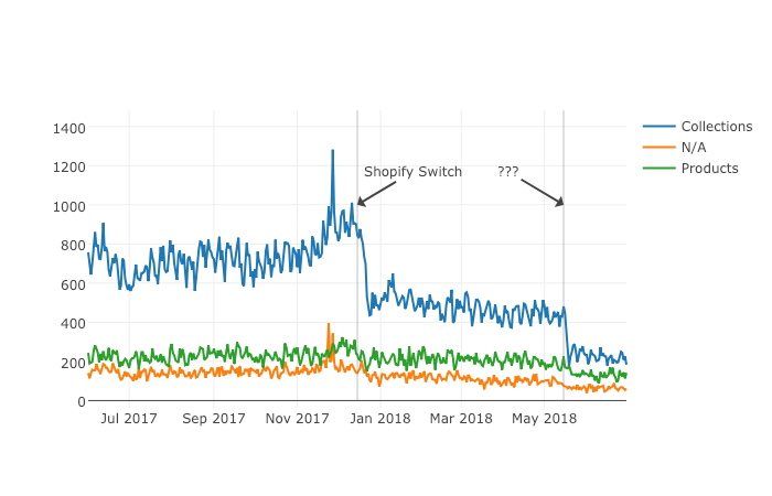
Last June we signed up a client that moved from Ecommerce V3 to Shopify and the SEO traffic took a big hit. The owner set up 301 redirects between the old and new sites but made a number of unwise changes like merging a large number of categories and rewriting titles during the move. When traffic drops, some parts of the site underperform while others don’t. I like to isolate them in order to 1) focus all efforts on the underperforming parts, and 2) learn from the parts that are doing well. I call this analysis the “Winners vs Losers” analysis. Here, winners are the parts that do well, and losers the ones that do badly.
A visualization of the analysis looks like the chart above. I was able to narrow down the issue to the category pages (Collection pages) and found that the main issue was caused by the site owner merging and eliminating too many categories during the move. Let’s walk over the steps to put this kind of analysis together in Python. You can reference my carefully documented Google Colab notebook here. Getting the dataWe want to programmatically compare two separate time frames in Google Analytics (before and after the traffic drop), and we’re going to use the Google Analytics API to do it. Google Analytics Query Explorer provides the simplest approach to do this in Python.
First, let’s define placeholder variables to pass to the APImetrics = “,”.join([“ga:users”,”ga:newUsers”]) dimensions = “,”.join([“ga:landingPagePath”, “ga:date”]) segment = “gaid::-5” # Required, please fill in with your own GA information example: ga:23322342 gaid = “ga:23322342” # Example: string-of-text-here from step 8.2 token = “” # Example https://www.example.com or http://example.org base_site_url = “” # You can change the start and end dates as you like start = “2017-06-01” end = “2018-06-30” The first function combines the placeholder variables we filled in above with an API URL to get Google Analytics data. We make additional API requests and merge them in case the results exceed the 10,000 limit. def GAData(gaid, start, end, metrics, dimensions, segment, token, max_results=10000): “””Creates a generator that yields GA API data in chunks of size `max_results`””” #build uri w/ params api_uri = “https://www.googleapis.com/analytics/v3/data/ga?ids={gaid}&”\ “start-date={start}&end-date={end}&metrics={metrics}&”\ “dimensions={dimensions}&segment={segment}&access_token={token}&”\ “max-results={max_results}” # insert uri params api_uri = api_uri.format( gaid=gaid, start=start, end=end, metrics=metrics, dimensions=dimensions, segment=segment, token=token, max_results=max_results ) # Using yield to make a generator in an # attempt to be memory efficient, since data is downloaded in chunks r = requests.get(api_uri) data = r.json() yield data if data.get(“nextLink”, None): while data.get(“nextLink”): new_uri = data.get(“nextLink”) new_uri += “&access_token={token}”.format(token=token) r = requests.get(new_uri) data = r.json() yield data In the second function, we load the Google Analytics Query Explorer API response into a pandas DataFrame to simplify our analysis. import pandas as pd def to_df(gadata): “””Takes in a generator from GAData() creates a dataframe from the rows””” df = None for data in gadata: if df is None: df = pd.DataFrame( data[‘rows’], columns=[x[‘name’] for x in data[‘columnHeaders’]] ) else: newdf = pd.DataFrame( data[‘rows’], columns=[x[‘name’] for x in data[‘columnHeaders’]] ) df = df.append(newdf) print(“Gathered {} rows”.format(len(df))) return df Now, we can call the functions to load the Google Analytics data. data = GAData(gaid=gaid, metrics=metrics, start=start, end=end, dimensions=dimensions, segment=segment, token=token) data = to_df(data) Analyzing the dataLet’s start by just getting a look at the data. We’ll use the .head() method of DataFrames to take a look at the first few rows. Think of this as glancing at only the top few rows of an Excel spreadsheet. data.head(5) This displays the first five rows of the data frame. Most of the data is not in the right format for proper analysis, so let’s perform some data transformations. First, let’s convert the date to a datetime object and the metrics to numeric values. data[‘ga:date’] = pd.to_datetime(data[‘ga:date’]) data[‘ga:users’] = pd.to_numeric(data[‘ga:users’]) data[‘ga:newUsers’] = pd.to_numeric(data[‘ga:newUsers’]) Next, we will need the landing page URL, which are relative and include URL parameters in two additional formats: 1) as absolute urls, and 2) as relative paths (without the URL parameters). from urllib.parse import urlparse, urljoin data[‘path’] = data[‘ga:landingPagePath’].apply(lambda x: urlparse(x).path) data[‘url’] = urljoin(base_site_url, data[‘path’]) Now the fun part begins. The goal of our analysis is to see which pages lost traffic after a particular date–compared to the period before that date–and which gained traffic after that date. The example date chosen below corresponds to the exact midpoint of our start and end variables used above to gather the data, so that the data both before and after the date is similarly sized. We begin the analysis by grouping each URL together by their path and adding up the newUsers for each URL. We do this with the built-in pandas method: .groupby(), which takes a column name as an input and groups together each unique value in that column. The .sum() method then takes the sum of every other column in the data frame within each group. For more information on these methods please see the Pandas documentation for groupby. For those who might be familiar with SQL, this is analogous to a GROUP BY clause with a SUM in the select clause# Change this depending on your needs MIDPOINT_DATE = “2017-12-15” before = data[data[‘ga:date’] < pd.to_datetime(MIDPOINT_DATE)] after = data[data[‘ga:date’] >= pd.to_datetime(MIDPOINT_DATE)] # Traffic totals before Shopify switch totals_before = before[[“ga:landingPagePath”, “ga:newUsers”]]\ .groupby(“ga:landingPagePath”).sum() totals_before = totals_before.reset_index()\ .sort_values(“ga:newUsers”, ascending=False) # Traffic totals after Shopify switch totals_after = after[[“ga:landingPagePath”, “ga:newUsers”]]\ .groupby(“ga:landingPagePath”).sum() totals_after = totals_after.reset_index()\ .sort_values(“ga:newUsers”, ascending=False) You can check the totals before and after with this code and double check with the Google Analytics numbers. print(“Traffic Totals Before: “) print(“Row count: “, len(totals_before)) print(“Traffic Totals After: “) print(“Row count: “, len(totals_after)) Next up we merge the two data frames, so that we have a single column corresponding to the URL, and two columns corresponding to the totals before and after the date.
We have different options when merging as illustrated above. Here, we use an “outer” merge, because even if a URL didn’t show up in the “before” period, we still want it to be a part of this merged dataframe. We’ll fill in the blanks with zeros after the merge. # Comparing pages from before and after the switch change = totals_after.merge(totals_before, left_on=”ga:landingPagePath”, right_on=”ga:landingPagePath”, suffixes=[“_after”, “_before”], how=”outer”) change.fillna(0, inplace=True) Difference and percentage changePandas dataframes make simple calculations on whole columns easy. We can take the difference of two columns and divide two columns and it will perform that operation on every row for us. We will take the difference of the two totals columns, and divide by the “before” column to get the percent change before and after out midpoint date. Using this percent_change column we can then filter our dataframe to get the winners, the losers and those URLs with no change. change[‘difference’] = change[‘ga:newUsers_after’] – change[‘ga:newUsers_before’] change[‘percent_change’] = change[‘difference’] / change[‘ga:newUsers_before’] winners = change[change[‘percent_change’] > 0] losers = change[change[‘percent_change’] < 0] no_change = change[change[‘percent_change’] == 0] Sanity checkFinally, we do a quick sanity check to make sure that all the traffic from the original data frame is still accounted for after all of our analysis. To do this, we simply take the sum of all traffic for both the original data frame and the two columns of our change dataframe. # Checking that the total traffic adds up data[‘ga:newUsers’].sum() == change[[‘ga:newUsers_after’, ‘ga:newUsers_before’]].sum().sum() It should be True. ResultsSorting by the difference in our losers data frame, and taking the .head(10), we can see the top 10 losers in our analysis. In other words, these pages lost the most total traffic between the two periods before and after the midpoint date. losers.sort_values(“difference”).head(10)
You can do the same to review the winners and try to learn from them. winners.sort_values(“difference”, ascending=False).head(10) You can export the losing pages to a CSV or Excel using this. losers.to_csv(“./losing-pages.csv”) This seems like a lot of work to analyze just one site–and it is! The magic happens when you reuse this code on new clients and simply need to replace the placeholder variables at the top of the script. In part two, we will make the output more useful by grouping the losing (and winning) pages by their types to get the chart I included above. The post Using Python to recover SEO site traffic (Part one) appeared first on Search Engine Watch. from https://searchenginewatch.com/2019/02/06/using-python-to-recover-seo-site-traffic-part-one/
0 Comments
Leave a Reply. |

AuthorPleasure to introduce my self i am Sean Webb i am 27 years old from Manchester, UK.I am doing affiliate marketing and have spend lots of time learning how to rank easy to medium competition keywords. I have recently started PPL and Video Marketing and learning more about it. ArchivesNo Archives Categories |


 RSS Feed
